Art of the DBA Rotating Header Image

partitioning

Sharing the Load

Businesses have always struggled with the high cost of relational database servers, both from a hardware and licensing perspective, because current RDBMS platforms take the approach that you will have one or two powerhouse servers handling your data workload.  While this has been the commonly accepted practice, the evolution of the cloud and better distributed computing architectures have given rise to new approaches for data storage and processing.  Now businesses are rethinking their approach to infrastructure with these new approaches, finding ways to provide better performance and higher availability all at a lower price point.

Non-relational data stores embrace this new approach with how they cluster.  Designed in response to the single, super-pricey database server, non-relational systems take the approach of clustering many inexpensive servers into one database.  This is sold as having many advantages to businesses, such as:

  • Horizontal scalability, allowing business to better adapt to growing workloads.  Need more power? Just add another commodity hardware server, you’re not trapped by the box you bought last year.

  • Distributed data across many machines, making the database more available and increasing the durability against failure.  Think of it as RAID for your data, so that if one box goes down, the system is still up and you just need to replace the one failed box.

  • Costs are lower and more manageable.  Well, at least more manageable, where you can buy only the computing power you need and grow incrementally over time.  However, there’s a lot of factors (from virtualization to overall hardware costs) that make the total price point versus a beefy relational server fairly comparable.

It’s certainly a departure from how we’ve dealt with relational platforms to date (though I’m super intrigued by Google’s F1 database).  There are some definite advantages, but most tech people look at this and say “Well, that sounds fancy, but does it blend?”  And by blend, we mean work.  The answer has actually been around for some time now and many large businesses already use it in their relational databases:  partitioning.

Partitioning is a concept we’ve had in the relational world for some time now (and feel free to look at my partitioning posts for more info).  Even before the major RDBMS platforms introduced their own partitioning functionality, DBAs would partition data out into different tables and bring them together as a view (commonly known as partitioned views).  What the non-relational folks do is take it a step further, saying that instead of just partitioning your data across different disks, why not distribute it across different computers?  By doing that, businesses not only get to spread the workload across all these computers, but their data availability is no longer dependent on a single OS/application instance.

Of course, what this means is that non-relational data stores still need some way to determine how data is partitioned.  Remember last week when I talked about all non-relational stores being key/value stores?  Well, those keys become even more important because they become the partitioning key (also called a shard key, by some), the value that non-relational platforms use to divvy up the data between its partitions.  Now, most of these datastores will analyze the key values and attempt to balance that data as evenly as possible, but it’s something you need to be aware of when modelling out your data.  A poorly chosen partition key could mean you’re negating your cluster advantage because your data will end up in one or two nodes.  We’ll come back to this in a bit.

At this point we should talk a bit about the CAP Theorem.  This bit of computer science was introduced back in 2000 and conceptually defines the limitations of a distributed computing system.  The gist of it is that, while we’re trying to accomplish all these wonderful things, any clustered platform cannot guarantee:

  • Consistency (That all the data on all the nodes is the same)

  • Available (That all the data is the same on all the nodes)

  • Partition Tolerant (That the application will remain up despite the loss of one of its partitions)

Commonly, you’ll hear people say that you can only have two out of these three things at any time.  What this means to non-relational platforms is that, since they’re all designed to be partition tolerant with their clustered nodes, we have to chose between being consistent or available.

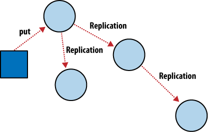
This is where eventual consistency comes in to play.  See, the problem with our clusters is that we still have the laws of physics involved.  When data is written and that data is distributed across multiple nodes, then there is a matter of time where data has to be communicated across a network and written to disks in different computers.  Most non-relational systems take the availability path here, meaning that data will be offered up from the various nodes, even if it’s not all up to date.  The idea is that it will be eventually consistent, but you might have to wait a bit.

Now our relational brains might kick back on us.  “Shouldn’t our data be 100% accurate all the time!?!?”  ACID compliance, right?  It depends!  Once again, we have to ask ourselves what data is being stored in our database.  Much of this detail only needs to be accurate at a point in time within an application, once it gets into the database we have a little more time before we have to deal with it.  If not, you might consider using a relational database for your data.  It’s all about using the right tool for the job.

One big concern coming out of this distributed model is the question of backups.  Non-relational folks will tell you that backups for disaster recovery aren’t really necessary because you have it built in.  However, most DBAs I know (and I’m one of them) will tell you that disaster recovery and high availability are not the same thing.  And because of the distributed nature, backups become really complex.  So you have to ask yourself when designing or implementing one of these solutions, how will you handle this?  In some cases, it might be a simple matter of backing up the files, but my research so far has shown that this requires an operating system file lock in order to keep things consistent.  Which means you stop your application (i.e., no hot database backups).  There might be other alternatives, either available or in development (the vendors of these platforms recognize the gap), but be aware that it will be a question you have to address.

The key takeaway for this post is that the distributed nature of non-relational systems is a huge advantage for them, but it has some hurdles to overcome.  It’s simply not a magic bullet to all your data problems.  Again, the theme here is using the appropriate tools for the appropriate purposes.  Recognizing the strengths and weakness is key to knowing when you should use a tool and, because NoSQL is a hot trend, it’s vital to understand it in order to properly guide your company’s conversations around the technology.

Next up, I want to talk about how non-relational systems leverage this dispersed architecture for querying and analyzing data.  It’s a strong offering, but not always fully understood.  Hopefully these last two posts are getting you interested in this realm of data management, but remember I’m only touching the surface here.  NoSQL is as deep (though not nearly as mature) as the RDBMS world and there’s a lot more learning than I can provide here.

A Heap of Trouble

A couple weeks ago I came across an interesting flaw in SQL Server partitioning which was causing one of my tables to balloon in size.  Essentially, we found that this large table in one of our databases had a lot of empty pages in it, pages that usually got cleaned up by the SQL Server engine.  Unfortunately these pages were not getting removed and this 2 billion row table was about triple the size it should have been.

I won’t focus on the table to much, but there were two elements that created this problem: the table was a heap and the partition key was volatile (got updated frequently).  I’m not yet sure if it’s a case of forward pointers or what other mechanic within SQL Server is behind this, but the result is that when we start moving data in a heap across partitions by changing the partition key, pages the data occupied were left behind and empty in the old partition.

To test it, I built a basic heap table partitioned on an integer, then stuffed it with 1000 rows.  I then queried some of the DMVs to see what the layout of the data was:

Partition 2 has 1000 rows in it, occupying 150 pages, exactly as we would expect.  Average page use is ~83.74%, so fairly full.  All in all, not unsurprising.  What happens, though, if we change the partition key value on those 1000 rows and move it to partition 3?

The 150 pages that the data used in partition 2 are still there!  And we now also are using 143 pages in partition 3!  The result of all this is that even though we’re not duplicating data, we’re duplicating space.  Normally, SQL Server will detect these empty pages and remove them, but in this case they are not identified as empty.

What would happen if, instead of updating our data, what happens if we simply delete the rows?

Even though we removed all our data from partition 2, those pages are still out there occupying space(note the avg_page_space_used_in_percent field).  Obviously, this can quickly spiral out of control and become a major issue.

I did go through all these tests with a clustered index on the table and the results were much more positive.  When I moved data from one partition to the next or deleted rows, the pages the data occupied were removed as expected, keeping the total size of the table down.

There are a couple lessons learned from this:

  1. Heaps are trouble!  Based on the evidence we have here, it’s fairly evident that using a heap table causes all sorts of problems with partitioning.  There are reasons the best practice of using clustered indexes in SQL server exists, this being one of them.
  2. Do not use a volatile partition key!  Keep in mind that when we partition, we’re managing the physical structure under our table.  In general, we want to avoid moving data around on our disk.  If we choose a partition key that changes a lot, we’re creating a situation where our data moves around unnecessarily, which can cause us other problems even with a clustered index in place.
  3. Design is vital!  The problems we had were created initially many years ago.  At the time, things looked fine and there weren’t any noticeable issues.  It wasn’t until much later, when the table had grown to several billion rows, that we had problems.  You need to take care in designing out your structures, because fixing very large tables is weeks(if not months) of coordinated work and can require significant downtime to implement.

So there it is.  I’m not sure if this is intended behavior or just an oversight.  Most of the folks I talked to regarding this had not encountered this before, which is not unsurprising.  The original table design violates several best practices.  However, I do want to make people aware of this and I plan on filing a Connect item regarding this once I’ve had a chance to bounce it off a few more SQL brains.

For those interested, the scripts to reproduce my testing are:

Process of Elimination

I never expected to talk as much about partitioning as I have so far this year. The tally is currently at six, with at least two more in the works. It’s a hot topic due to partitioning still being a mystery to a lot of folks and I’m glad I’ve been able to pull back the curtain a little bit.  However, there’s still some things not understood very well.

One of these is partition elimination. Heck, up until I really started studying partitioning, I didn’t understand it very well either. Just like many others out there, I thought that once you partitioned a table, all your queries would suddenly become faster because the engine would only look at the needed partitions. While SQL Server tries to do this, the reality of when partition elimination actually occurs is not quite as cool.

To figure out how partition elimination works, we only have to look at our query plans. Let’s crack open the demo I use in my partitioning presentation and take a look. As a quick recap, I use a basic orders table that is partitioned on an incrementing integer primary key:

Now let’s run a simple SELECT to query data out and capture the query plan that results:

select * from orders
where order_id between 11000 and 15000

Nothing complex here and nothing complex in the query plan. You’ll see the expected clustered index seek. What’s key is to look at the properties (F4) of your operator to see how your partitions are being used:

These two property values give us all the answers when it comes to partition elimination. First, Partition Count tells us that the engine only retrieved a single partition for our query. Actual Partitions gives us the partitions (in this case, partition 3) that were actually accessed. Great! In this case, by querying order_id, we were able to take advantage of our partitioning.

What if we use a different field, will SQL still try to take advantage of the partitioning? It depends on whether or not the partitioning key is used in any part of the query. We’ll go ahead and add an index on order_date (which will be partitioned aligned) and query to get the total order amount for date range:

select sum(order_amount)
from orders
where order_date between '1/1/2012' and '2/1/2012'

Now, this plan is a little more interesting, so let’s take a look at it, focusing on the two places where we hit the table:

You’ll note that the query has to use a key lookup to complete the query. This is because we have an index on order_date, but it doesn’t include the order amount, so the engine has to go back to the table using the clustered index to find our data. Let’s now look at the properties for each of these operators:

Where are the partition properties for the index seek? Since the query can’t make use of partitioning for this part of the query, the properties aren’t listed. However, the key lookup (which makes use of the clustered index and, therefore, our partitioning scheme) does show that we accessed only partition number 3.

What if we go a step further and alter our index on order_date to include order_amount, removing the need to do a key lookup in the query? Let’s take a look:

By detailing that the query accessed eight partitions (1..8), we see that the engine tried to use the partitioning.  Since the partitioning key wasn’t directly involved, it ended up seeking across the entire index anyway.

To wrap it all up, let’s look at the performance of our order_amount queries:

  • Query cost on index without include: 2.63403
  • Query cost on index with include: 0.0276018

So even without using our partitioning, including the order_amount is still much faster than having to do a key lookup.

Overall, partition elimination can be a helpful tool in the engine’s toolbox. As your data sets get larger and larger, it can improve your performance, but only if you understand how the engine uses partitions. Sometimes, however, it’s better to take a different approach.  Don’t go and rewrite all your queries simply to get your partitioning key involved, because it may not help. Always do a careful analysis of what’s going on under the covers before making any tuning decisions.

Upcoming Presentations

More on the how later, but I wanted to let folks know about some presenting I’ll be doing over the next couple of months. I’m extremely excited for all of this speaking and the opportunities to share with the SQL Server community.

My partitioning presentation, Eating the Elephant, is now slotted for three upcoming events:

  • PASS Virtual Performance Chapter – For those following this group, Jes Borland-Schulz(b|t) did a great presentation on filegroups last week. Partitioning will be a natural follow up to this topic and I’ll be presenting to this group on March 22.
  • PASS Virtual Data Architecture Chapter  – Tom LeBlanc(b|t) asked me to give this presentation in April 19 after we talked at SQL Saturday #104 in Colorado Springs.
  • SQL Rally in Dallas – Seriously, I’m giddy about this. The SQL Community selected me as part of the Community Choice vote and I’ll be giving this presentation sometime during the conference. For those of you interested, I blogged about the first SQL Rally last year. It’s a great event, much cheaper than the Summit, and was a fantastic boost for my career. Even if you don’t come to see my presentation (I forgive you), you really should go.

I’m extremely excited and honored that people want to hear me speak. Presenting is a lot of fun for me and very rewarding, both on a personal and professional level. It’s a vicious cycle, too, because while I’m giving the same presentation three times over the next three months, I’ve already got 2-3 more presentation ideas bubbling around in my head that I plan to give by the end of the year. Stay tuned, 2012 is turning out to be pretty awesome!

Excuse me sir, are you using that partition?

So last week we had to puzzle out a little weirdness at work. One of our development teams is working to implement partitioning and they came to us about their scheme. They had applied a partitioning scheme, but it wasn’t being used by their queries. Their scheme was pretty simple, but the oddity was that they had partitioned on a nvarchar(10) field. Best practice is to use an integer, though I’ve seen date fields used as well. Though I knew that you could partition on a character field, I usually avoided it.

Now, using an nvarchar field shouldn’t have altered the query process that much, right? This is where it got odd, because what we were seeing was that a query on that partition scheme was still querying across all partitions. Here’s the query and what we were seeing in the query plan:

One of the advantages of partitioning is to improve query performance with range scans, so that the engine will only query across partitions. However, even though our query was specifically using the partition key, the engine was still querying across all partitions for its result. And we were specifically using a nvarchar value for the query criteria, so it shouldn’t be doing any sort of conversion, right? Well, that’s where you (and we, as well) would be wrong. We tried the query again, this time with an explicit conversion to nvarchar(10):

Bang! By converting it to the same datatype as the partition key, the query engine can now properly take advantage of our partitioning. The results are further reinforced by looking at the query costs of our two queries:

  • Query 1: 0.0131291
  • Query 2: 0.0032831

What just happened?

What’s going on behind the scenes is that in query 1 our predicate datatype does not match the datatype of our partition key. The SQL Server engine sees the query predicate of CUSTOMERID=N’2’ as an nvarchar(4000), not as an nvarchar(10). Just take away the “N” in front of our string value and have it declared as a character string and force an implicit conversion. Then, if you look at the query operator, you’ll see SQL Server do a CONVERT_IMPLICIT to nvarchar(4000), not a nvarchar(10).

I also went through this exercise using varchar as my datatype and got the same results. If I simply declared the predicate as CUSTOMERID=’2’, my query would seek across all partitions. If I used CUSTOMERID=convert(varchar(10),’2’), then I would only have the one active partition.

I’m not sure if this is a bug or working as intended, but there’s definitely a couple of lessons we can take from this:

  1. To best take advantage of querying across partitions, you need to make sure your query criteria is explicitly the same datatype as your partition key. Otherwise, the engine can’t make use of your partitioning.
  2. Obviously character strings have some weirdness about them for partitioning, so it’s best to avoid them for partition keys.
  3. Mike is weird for geeking out about this stuff. Seriously. My co-workers gave me some odd looks as we were puzzling this out.


Monday Scripts – Getting Partition Information

I’m going to follow up my post on partitioning with a query I wrote while implementing the partitions and cleaning up the empty ones. One of the issues I ran in to was clearly seeing each partition’s range and the number of rows within it. These two questions are answered in different places in the catalog views, sys.partition_range_values and sys.partitions. To build this out, I started with a nice little query from Derek Dieter, adding in a couple joins to get me to sys.partitions. Here’s the result!

select 
	t.name as TableName
	, ps.name as PartitionScheme
	, pf.name as PartitionFunction
	, p.partition_number
	, p.rows
	, case 
		when pf.boundary_value_on_right=1 then 'RIGHT' 
		else 'LEFT' 
	  end [range_type]
	, prv.value [boundary]
from sys.tables t
    join sys.indexes i on t.object_id = i.object_id
    join sys.partition_schemes ps on i.data_space_id = ps.data_space_id
    join sys.partition_functions pf on ps.function_id = pf.function_id
    join sys.partitions p on i.object_id = p.object_id and i.index_id = p.index_id
    join sys.partition_range_values prv on pf.function_id = prv.function_id and p.partition_number = prv.boundary_id
where i.index_id < 2  --So we're only looking at a clustered index or heap, which the table is partitioned on
order by p.partition_number

My Partitioning Odyssey

Recently I had my first real experience with SQL Server partitioning. I had known about it, sure, but most of it was general understanding of the concepts and no real practical experience. Well, all of that changed last month when I successfully partitioned a table with several billion (with a “B”) rows to help get a grip on an application that was slipping out of control. I’d like to walk you through the process to try and help you with any partitioning you intend to do.

That’s no moon!

First off, let’s look at the problem. Like I said, we had a big table, but what does that mean? Well, here’s the hard stats from sp_spaceused:

19,600,710,213 rows
~759 GB reserved space
~432 GB data space
~326 GB index space
~120 MB free space

Yeah, pretty big right? I mean, at 759 GB, this one table was bigger than most databases that I’ve worked with. Structurally, it wasn’t all that complex, though, as it had 3 fields, a composite clustered primary key, and a non-clustered index. However, even with it being very narrow, the size of it prevented us from being able to do any maintenance. And it was almost impossible to properly identify and roll off any data, so our problem was only going to get worse.

How do you eat an elephant?

Based on some of my reading, I was pretty sure partitioning was our way out, but I needed more information. A couple weeks of research later, I came up with the following links that really helped me “get it”:

Partitioned Tables and Indexes in SQL Server 2005
Simple Talk-Partitioned Tables in SQL Server 2005
Kimberly Tripp Web Cast
SQLServerpedia Partitioning article

The first thing I got out of all these articles was why you would want to do partitioning on a table this size:

  • Ability to rebuild/manage indexes as each partition could be rebuild separately.
  • Increased performance for reads based on better data targeting by the query engine, as it should only retrieve needed partitions.
  • Increased performance on all queries, as we would be able to maintain the indexes on the table.
  • Possible performance increase on inserts.
  • Ability to better archive off data as the table grows, thus being able to overall manage space on the server.

So what partitioning gives you is a way to manage the table in small chunks instead as one large object. Or a better way to think of it is the old cliché: How do you eat an elephant?

One bite at a time.

Now, there were also some key ground rules I learned about partitioning:

  • Table partitioning defines how the table will be physically stored
    • If partitioning a heap, then the partition field can be any field in the table since no field is involved in defining how the table is physically stored on disk.
    • If partitioning a table with a clustered index (like a primary key), then the partitioning field must be one of the fields included in the index, as the clustered index defines how the table is physically stored on disk.
  • You are always partitioning by RANGE. If you wish to partition on specific values, then your range declaration will be of that value.
  • Each partition is a physically separate entity, meaning that you can allocate partitions to different file groups within SQL Server. This would be the method of explicitly assigning parts of a table to specific disk locations.
  • SQL 2005 and 2008 are limited to 1000 partitions.

The first point was pivotal for me, as I had seen a bunch of examples where some guys had partitioned on a table field, and some on a clustered index field. Understanding that table partitioning revolves around how the table is physically stored on disk really made it all clear for me.

Planning time!

Armed with this knowledge, it was time to build out my partition structure. The first step was to figure out what I was going to partition on. The table was designed to store a value based on a combination of an individual id, representing a person, and a field id, detailing what type of data was being stored for that individual. Reviewing the ground rules, I knew you could only partition on one field and it must be part of that clustered index, so I was limited to selecting one of those fields. Your partitioning doesn’t have to be the entire clustered index, so using just one of these fields was fine. As the individual id values was pretty granular(about 1.6 billion distinct values), I went with that as my partitioning field.

Next up, I needed to decide on my ranges. The individual id was a numeric, auto-incrementing value, so this made it easy to establish a numeric range. The real question was how large to make each partition, since I wanted them small for manageability, but not to small so I would go over the 1000 partition limit. I ended up deciding on making each partition 5 million distinct individual ID values, which would mean roughly 50 million rows per partition (the individual id to assigned fields ratio was about 1 to 10).

With these two decisions made, I was able to write the following SQL code to create my function, scheme, and table(names have been changed to protect the troublesome):

create partition function pf_bigtable (int)
as range left for values();

declare @boundary int
declare @increment int

set @boundary = 5000000
set @increment = 5000000

while @boundary < 2000000000
begin
	alter partition function pf_bigtable() split range (@boundary)
	set @boundary = @boundary+@increment
end

create partition scheme ps_bigtable
as partition pf_ bigtable
all to ([PRIMARY]);

--Create new table
CREATE TABLE [dbo].[bigtable_p](
	[individualid] [int] NOT NULL,
	[fieldid] [int] NOT NULL,
	[valueid] [int] NOT NULL,
 CONSTRAINT [pk_bigtable_p] PRIMARY KEY CLUSTERED
(
	[individualid] ASC,
	[fieldid] ASC
) ON ps_recipidsv(individualid)
--NC index (created later)
CREATE NONCLUSTERED INDEX [ix] ON [dbo].[bigtable_p]
(
	[fieldid] ASC,
	[valueid] ASC
)

Notice that I used a looping statement to add in all my ranges to save myself the effort of explicitly declaring several hundred partitions.

Getting it in place

The biggest hurdle was partitioning out the table itself. This table was part of an OLTP system that needed to be up almost 24/7. We had a weekly maintenance window of 3 hours one night in the week, but that wasn’t enough time to apply this operation to the live table. Fortunately, we did have plenty of disk space.

What I did was pretty straightforward. I went ahead and created the table with the fully created partition scheme as described above, but empty of data. I also held off creating the non-clustered index. At this point I had an empty copy of my live table. With the help of one of the other guys on my team, we built a batch insert process to step through the live table and insert small batches of records (~6 million at a time) into the partitioned table, so we could build up about 99% of the data from the live table to our partitioned copy. Once we had gotten the bulk of the data inserted, I then created the non-clustered index. When this was completed, we then took the application offline to stop writes to the table, ran a final insert process to get all the new records we had missed since we created the non-clustered index, and then changed the table and index names, swapping the unpartitioned table with the partitioned one.

The initial copy actually took several days to complete, but we were able to have uninterrupted application service during the whole time. When the non-clustered index build was finished, we ended up having only 30 minutes of application downtime to catch everything up and swap the objects.

The finish line

So now that we got all this into place, it was time for us to see what the partitioning bought us. The first item on my list was seeing if I could rebuild the index on the table. By making use of the dm_db_index_physical_stats dynamic management function, I was able to write a script to rebuild each individual partition as necessary:

declare recscan cursor for
SELECT partition_number
FROM sys.dm_db_index_physical_stats (DB_ID(),OBJECT_ID(N'dbo.bigtable'), NULL , NULL, NULL)
where avg_fragmentation_in_percent >= 30;

declare @sql varchar(max)
declare @partnum varchar(10)

open recscan
fetch next from recscan into @partnum
while @@fetch_status = 0
begin
set @sql = 'alter index all on bigtable_p rebuild partition='+@partnum
exec(@sql)
fetch next from recscan into @partnum
end

close recscan
deallocate recscan

The initial run of this still took 8+ hours to complete, so not any real time savings there. However, since most of the table wasn’t getting affected (it was mostly inserts, very few updates), subsequent maintenance only took 5-15 minutes each run because only a handful of partitions actually needed to be addressed.

We also saw dramatic performance in the use of the application. SELECTs of the data were much faster, and the load process that did most of the inserting into the table saw upwards of a 150% speed increase.

Overall, this was a huge win for me and a fantastic learning experience. You can never really put something in your toolbag until you’ve actually been able to do it, and it’s not every day a challenge like this comes your way. However, this experience should also stress the necessity of planning, because we had to jump through a lot of hoops to get the partitions on this table after it had already grown to an unmanageable size. A lot of that effort could have been saved if someone had given some more thought to the amount of data flowing into this system.

Anyway, there’s my partitioning odyssey. I hope this was beneficial to you and if there’s anything that wasn’t clear or may have been missed, don’t hesitate to drop me a note and let me know!